Examples and applications

torchwavelets ships self-contained, reproducible examples. Each one downloads its (real) data on first use into ~/data/torchwavelets, renders a figure into docs/figures/, and prints the measured numbers. Everything runs on CPU with only PyTorch + numpy + matplotlib (plus scikit-learn and Pillow for the classification and photo examples):

pip install -e ".[examples]"       # torch, numpy, pywt + example deps
python examples/plot_transform_gallery.py
python examples/application_denoising.py
python examples/application_ecg.py
python examples/application_cifar10.py

script	application	data
plot_transform_gallery.py	visual tour of every transform	photograph (USC-SIPI)
application_denoising.py	image denoising, DWT vs DTCWT	photograph (USC-SIPI)
application_ecg.py	ECG denoising, SWT vs DWT	MIT-BIH record 100 (PhysioNet)
application_cifar10.py	image classification with scattering features	CIFAR-10

---

1. A tour of every transform

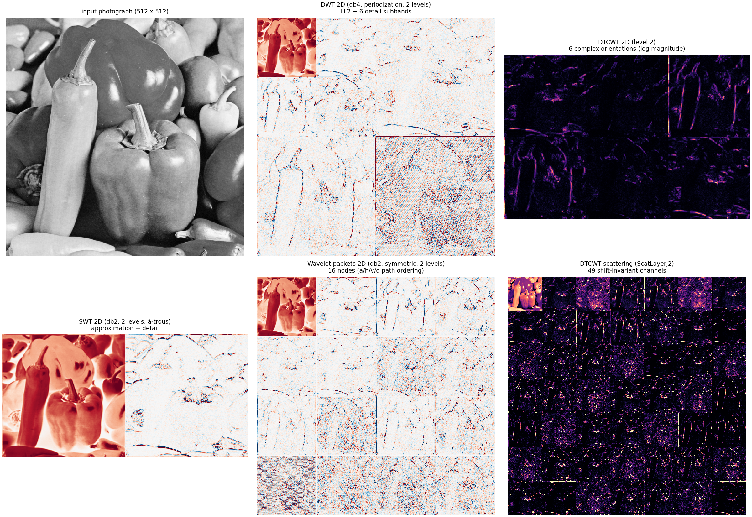
python examples/plot_transform_gallery.py applies the whole package to a real 512x512 photograph (the classic peppers test image): the critically sampled DWT, the six complex orientations of the DTCWT, the undecimated SWT, the full binary wavelet-packet tree, and the 49 shift-invariant channels of a two-scale DTCWT scattering layer.

What to look at:

• DWT 2D — three separable orientations (LH/HL/HH) per level; the energy concentrates along horizontal, vertical and diagonal edges.
• DTCWT 2D — six complex orientations at ±15°, ±45°, ±75°, giving directional selectivity and near shift invariance (no aliasing of the checkerboard kind).
• SWT 2D — the à-trous approximation and detail keep the full input resolution (no decimation), so fine features are never discarded.
• Wavelet packets 2D — 16 nodes of the quaternary tree (a/h/v/d path ordering, PyWavelets-compatible).
• DTCWT scattering — smoothed moduli of the bandpasses; the invariants are exactly shift-invariant at dyadic shifts.

---

2. Image denoising: DWT vs DTCWT

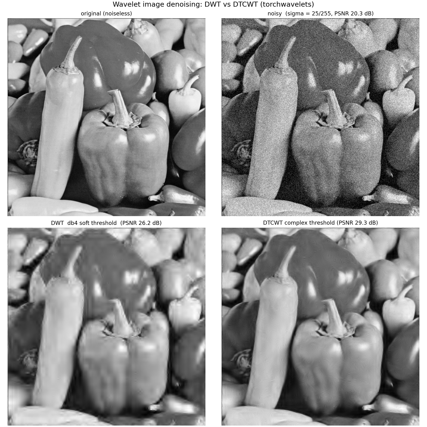
python examples/application_denoising.py corrupts the photograph with white Gaussian noise (σ = 25/255) and restores it by per-level soft thresholding of the wavelet coefficients — the same 3σ rule for both transforms:

• DWT (db4, 4 levels, periodization): real soft threshold sign(c) · max(|c| − λ, 0) per subband.
• DTCWT (near_sym_a / qshift_a, 4 levels): complex (Kingsbury) shrinkage W · max(1 − λ/|W|, 0) on the six orientation bandpasses.

method	PSNR
noisy (σ = 25/255)	20.3 dB
DWT, db4 soft threshold	26.2 dB
DTCWT, complex threshold	29.3 dB (+3.1 dB)

Why the DTCWT wins: its 2× redundancy and near shift invariance make the coefficients consistent — a feature's energy stays in a single orientation across nearby scales, so the complex threshold keeps it while the equivalent real-domain threshold spreads the attenuation across misaligned DWT coefficients. (Implementation detail worth knowing: the DTCWT coefficient noise floor is ≈3× lower than the DWT's, so per-level thresholds must be estimated from the actual coefficient statistics — the example measures them from a noise-only forward pass.)

---

3. ECG denoising: SWT vs DWT

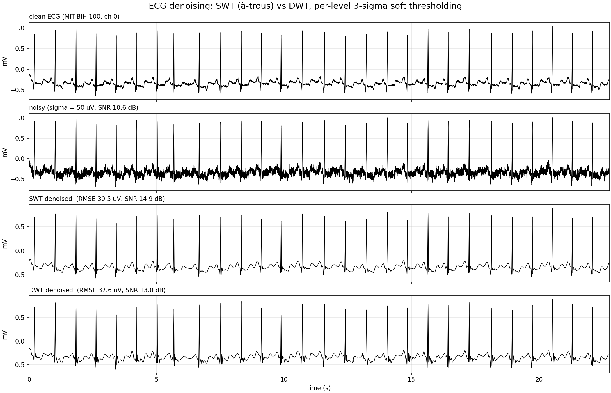
python examples/application_ecg.py takes a real 360 Hz electrocardiogram (MIT-BIH Arrhythmia record 100, channel 0, 8192 samples), adds 50 µV of white noise, and compares two wavelet denoisers under the same per-level 3σ soft thresholding:

• DWT (db4, 5 levels, symmetric) — critically sampled.
• SWT (db4, 5 levels, à-trous) — undecimated: every translation of the wavelet is kept at every scale.

method	RMSE	SNR
noisy (σ = 50 µV)	—	10.6 dB
DWT, soft threshold	37.6 µV	13.0 dB
SWT, soft threshold	30.5 µV	14.9 dB (+1.9 dB)

The SWT is more faithful because thresholded undecimated coefficients still correspond to every time instant — the denoised signal cannot develop the shift-consistency artefacts of the critically sampled reconstruction, and the QRS complexes survive with less distortion.

---

4. CIFAR-10 classification with scattering features

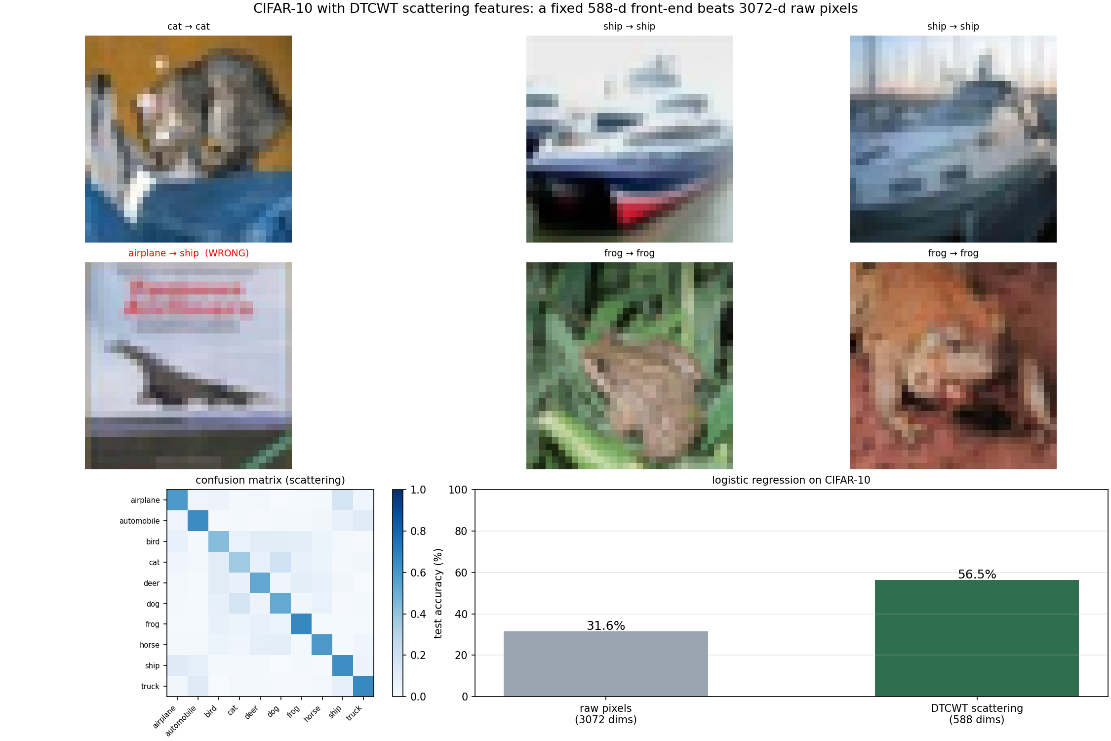
python examples/application_cifar10.py runs the classic Mallat recipe: a fixed, untrained DTCWT scattering front-end extracts locally shift-invariant features, and only a linear classifier is learned on top:

1. DTCWTScattering(J=2, max_order=2) on every 32x32 colour image → 147 invariants (order-0 lowpass, first-order paths (1,), (2,) and the second-order path (1,2), 6/18 orientations per channel).
2. 2×2 average pooling of each invariant → 588 dimensions per image.
3. Multinomial logistic regression (standardised features, lbfgs, converged).

Baseline: the same classifier on the 3072 raw pixels.

features	test accuracy
raw pixels (3072-d)	31.6 %
DTCWT scattering (588-d, untrained)	56.5 % (+24.9 points)

The front-end contributes no learned parameters: the gain comes from the scattering transform itself — modulus nonlinearities that are stable to deformations, and invariance that is built in rather than learned. This is the same recipe behind early deep "scattering networks" and still a strong baseline for small-data regimes.

5. Mixed-precision training with PyTorch Lightning

python examples/application_lightning.py trains a small CIFAR-10 classifier with PyTorch Lightning: a frozen torchwavelets front-end (a critically sampled DWT2D layer + a DTCWTScattering network, zero learned parameters) feeds a learnable MLP head. The script picks precision="16-mixed" on CUDA and "bf16-mixed" on CPU, and prints an audit of the dtype of every stage produced inside the Trainer's autocast context:

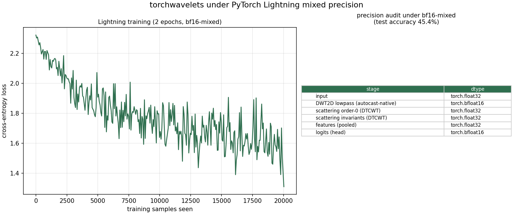
stage	dtype under bf16-mixed	why
input	float32	data loader
DWT2D lowpass	bfloat16	autocast-native: follows the Trainer precision
DTCWT scattering	float32	documented exception: no complex bf16 kernels; never breaks AMP
pooled features	float32	computed from the float32 scattering
head logits	bfloat16	linear layer runs in the autocast dtype

This is the precision-management contract of the package:

• DWT / SWT are built from plain conv2d/conv_transpose2d ops — output dtype == autocast dtype (bfloat16/float16/float32), and fp16/bf16/ fp32/fp64 inputs pass through unchanged outside autocast.
• DTCWT (1D/2D/3D), scattering layers and networks compute in float32 (half and bfloat16 inputs are promoted) and run in an autocast-disabled scope — torch.complex has no bf16 kernel, so this is the only way to be AMP-safe. The result is float32/complex64 regardless of the Trainer precision.
• Nothing requires torch.set_default_dtype; the module API resolves filters eagerly, so torch.compile and Lightning work together.

The companion test suite (tests/test_lightning.py) asserts exactly this for Trainer(precision="32-true"/"64-true"/"bf16-mixed") on CPU and "16-mixed" on CUDA, and checks gradients flow through both wavelet layers inside a Lightning training step.

---

Reproducibility

• Fixed seeds (torch.manual_seed, numpy.random.default_rng) — the numbers in this page are reproducible.
• Data is downloaded once and cached in ~/data/torchwavelets (photograph, CIFAR-10, MIT-BIH ECG); run the scripts from the repository root.
• Reference results (CPU, this repository at commit 6bf6a0a):

example	reference result
denoising	DWT 26.2 dB → DTCWT 29.3 dB
ECG	DWT 13.0 dB → SWT 14.9 dB SNR
CIFAR-10	raw 31.6 % → scattering 56.5 %
Lightning (bf16-mixed)	45.4 % test accuracy; DWT→bf16, DTCWT→fp32